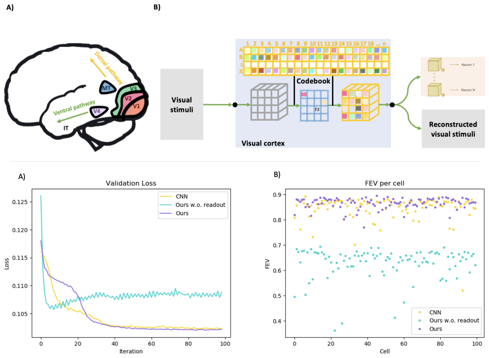
The question
Neurons in primary visual cortex (V1) each prefer edges at a particular orientation. Recognizing objects, though, requires features that stay the same when an object rotates. How the visual system gets from orientation-tuned neurons to rotation-invariant representations is still unclear.
CNN models of V1 already predict neural responses to natural images well. They capture the idea that many neurons do the same computation at different locations by splitting the final readout into a where part (a spatial mask) and a what part (feature weights). To handle rotation, earlier models built rotated copies of their filters by hand. Could a model instead learn a shared set of features, independent of each neuron’s preferred orientation, by being forced to use a discrete vocabulary?
What we did
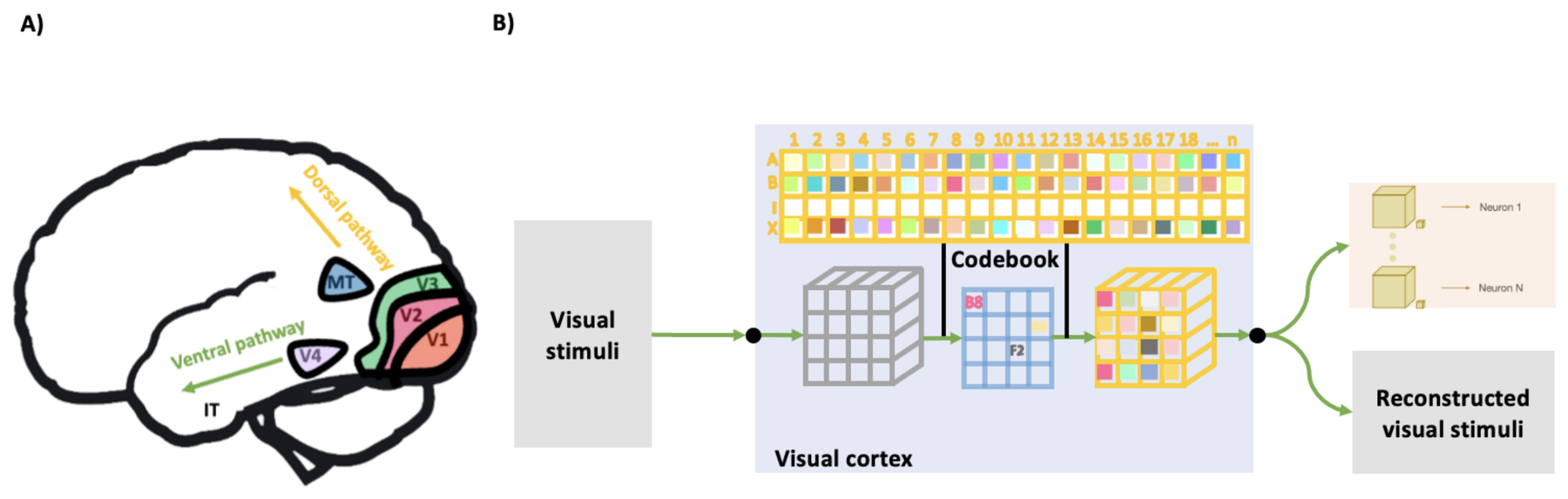
We built a model based on a vector-quantized autoencoder (VQ-VAE):
- An encoder turns the stimulus into a grid of feature vectors.
- Each vector is replaced by its nearest entry in a learned discrete codebook.
- The quantized features go down two branches. One decoder reconstructs the image. A factorized readout predicts each neuron’s response, using a spatial mask (where the neuron looks) times feature weights (what it responds to).
The model is trained on three goals at once: predict neural responses, reconstruct the stimulus, and keep the codebook entries close to the encoder’s outputs.
We tested it on a synthetic dataset: 100 model neurons responding linearly to 48 × 48 px Gaussian white-noise images. Performance was measured as the fraction of explainable variance explained (FEV; 1 is perfect) and the correlation between predicted and true responses.
What we found
1. Discrete codes predict neurons as well as a CNN
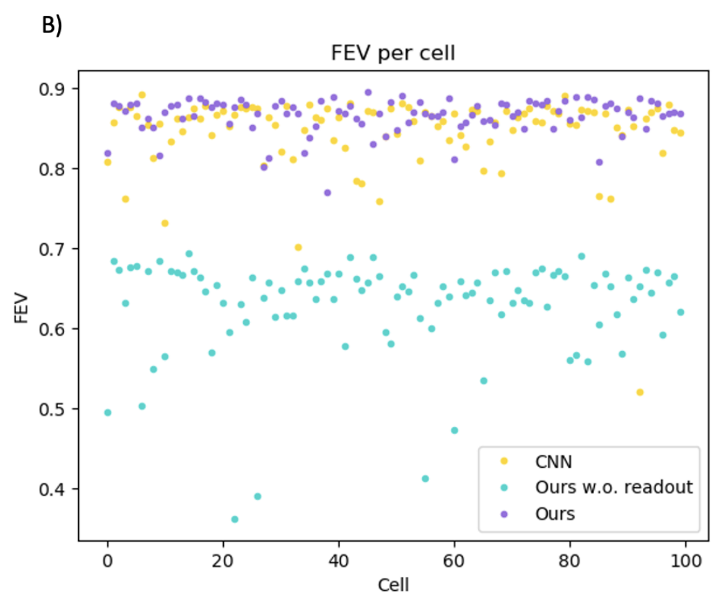
With a fraction of explainable variance of 0.86 and a correlation of 0.936, the discrete-codebook model matched a standard CNN (0.84 and 0.936). Forcing the model through a small vocabulary of features did not cost predictive accuracy.
| Model | FEV | Correlation |
|---|---|---|
| CNN | 0.84 | 0.936 |
| Ours without factorized readout | 0.63 | 0.838 |
| Ours | 0.86 | 0.936 |
2. Separating “where” from “what” is essential
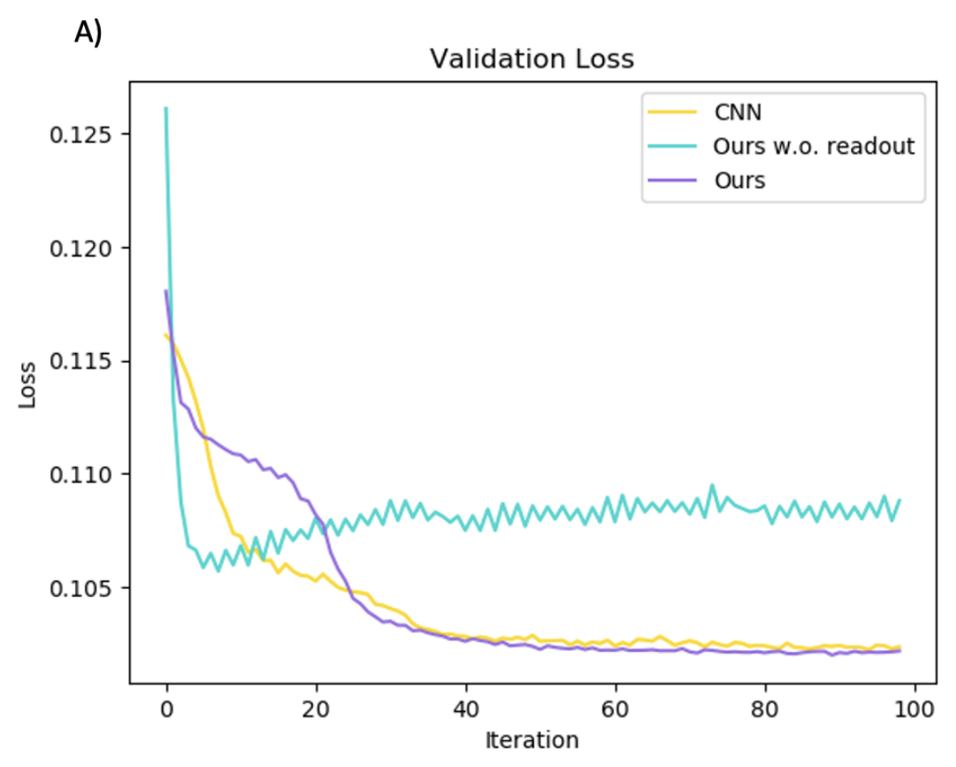
Without the factorized readout, performance dropped to an FEV of 0.63. The validation loss also stalled early and slowly rose. With it, the loss kept falling and leveled off alongside the CNN’s. Splitting each neuron’s readout into a spatial mask and feature weights is what lets the shared codebook serve all 100 neurons.
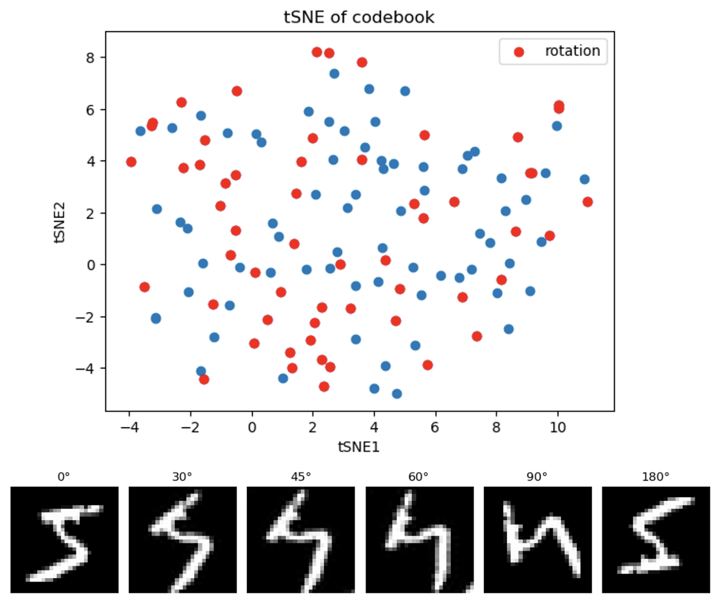
3. A first look at rotation in the codebook (preliminary)
As a first step toward the rotation question, we embedded the codebook entries for an image and for its rotated versions in two dimensions. This analysis is exploratory, and testing whether the codes are truly rotation-invariant is listed on the poster as future work. Next steps are real V1 recordings and a hierarchical codebook.
My take
Links
BibTeX
@misc{li2024visualneural,
  title        = {A Framework of Mapping Visual Stimulus to Neural Responses via
                  Discrete Latent Representation},
  author       = {Li, Chenyi and Ran, Xuming},
  howpublished = {Poster, NITMB Emerging Directions Workshop, Chicago, IL},
  year         = {2024}
}